# load packages
library(countdown)
library(tidyverse)
library(glue)
library(lubridate)
library(scales)
library(ggthemes)
library(gt)
library(palmerpenguins)
library(openintro)
library(ggrepel)

# set theme for ggplot2
ggplot2::theme_set(ggplot2::theme_minimal(base_size = 14))

# set width of code output
options(width = 65)

# set figure parameters for knitr
knitr::opts_chunk$set(
  fig.width = 7,        # 7" width
  fig.asp = 0.618,      # the golden ratio
  fig.retina = 3,       # dpi multiplier for displaying HTML output on retina
  fig.align = "center", # center align figures
  dpi = 300             # higher dpi, sharper image
)Data wrangling - III
Lecture 8
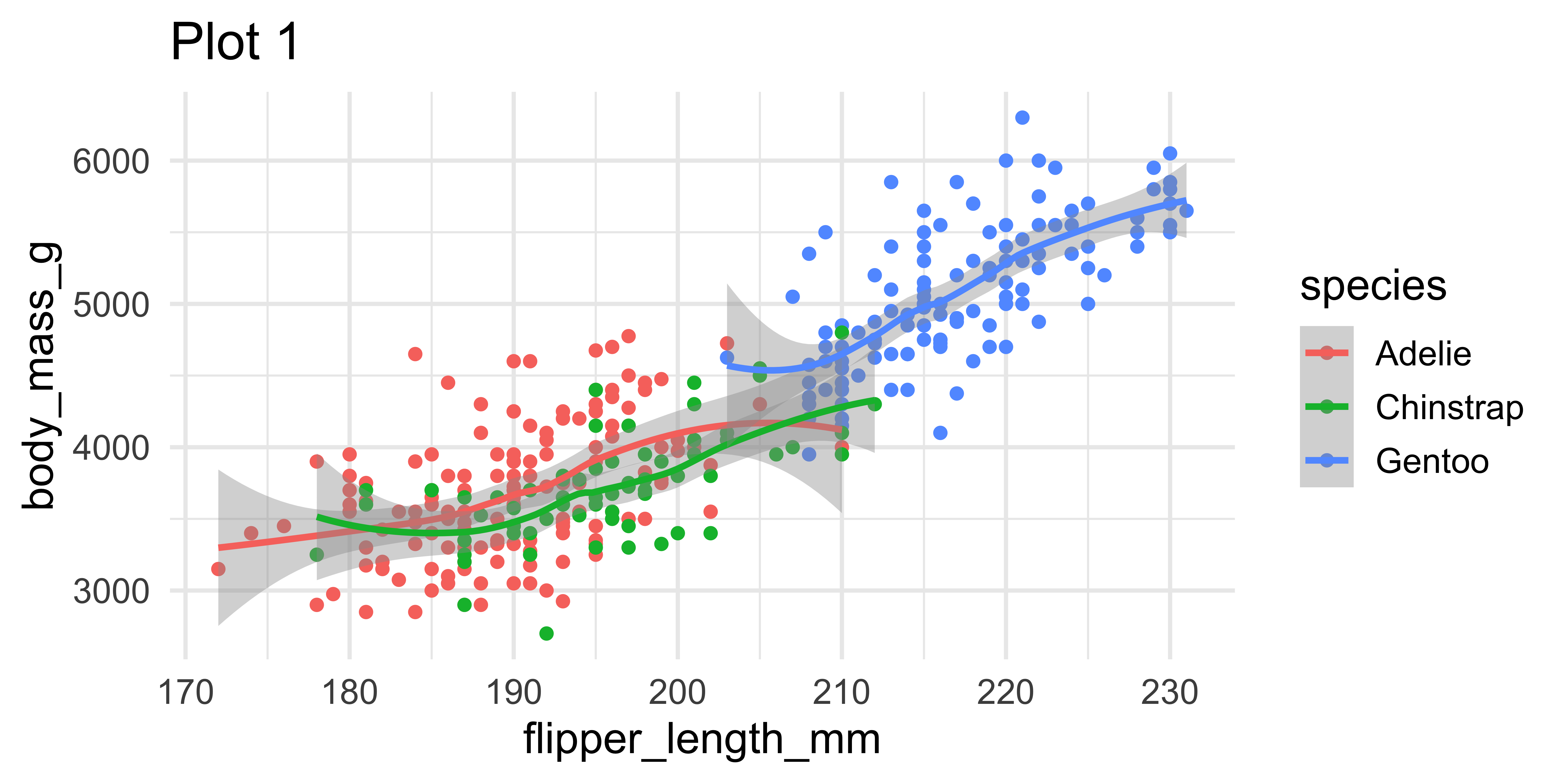
Missing values I
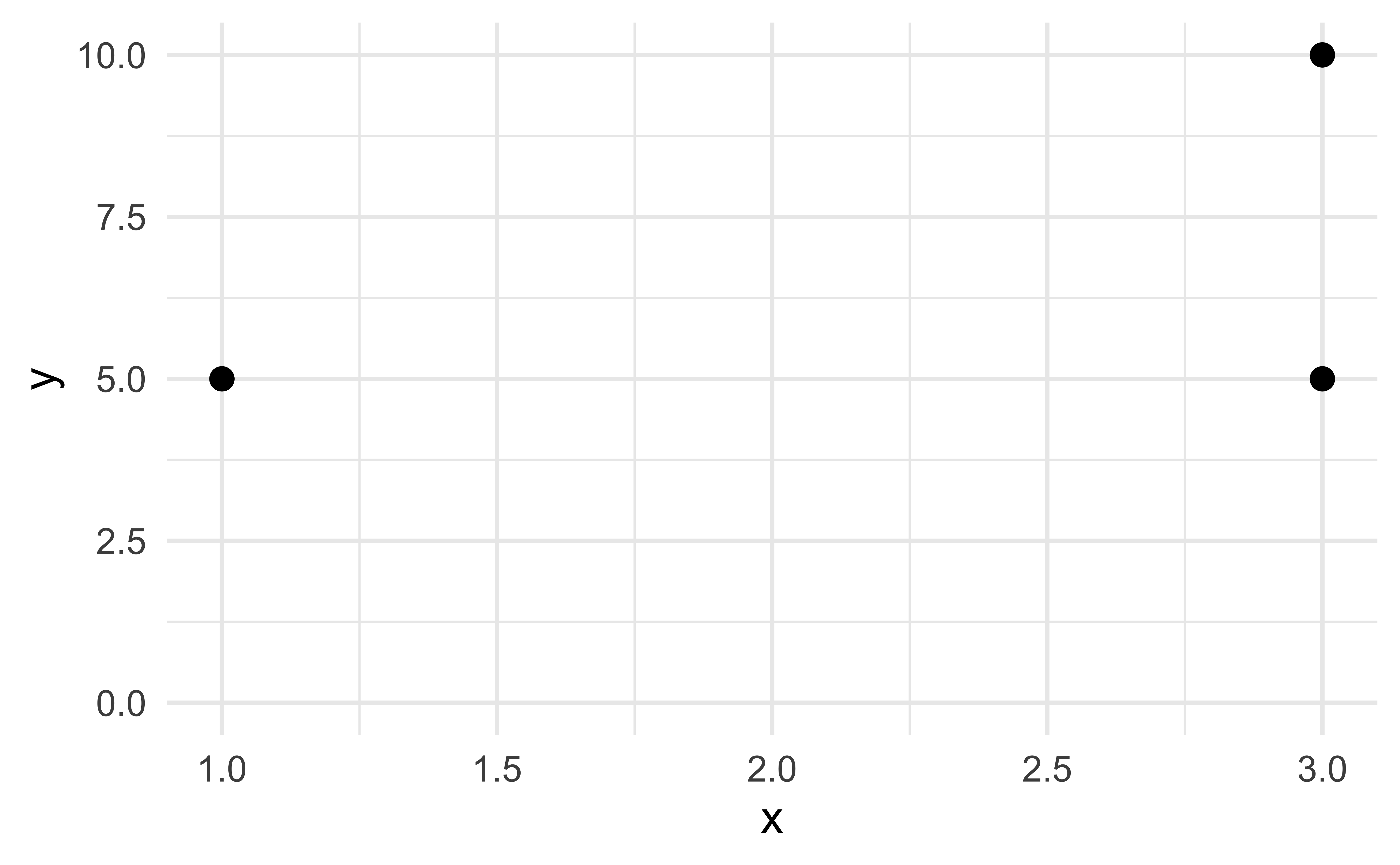
Missing values II
Missing values II
Is it ok to suppress the following warning? Or should you update your code to eliminate it?
Missing values II
Is it ok to suppress the following warning? Or should you update your code to eliminate it?
Warning: Removed 69 rows containing non-finite values
(`stat_boxplot()`).
Missing values II
Why doesn’t the following generate a warning?
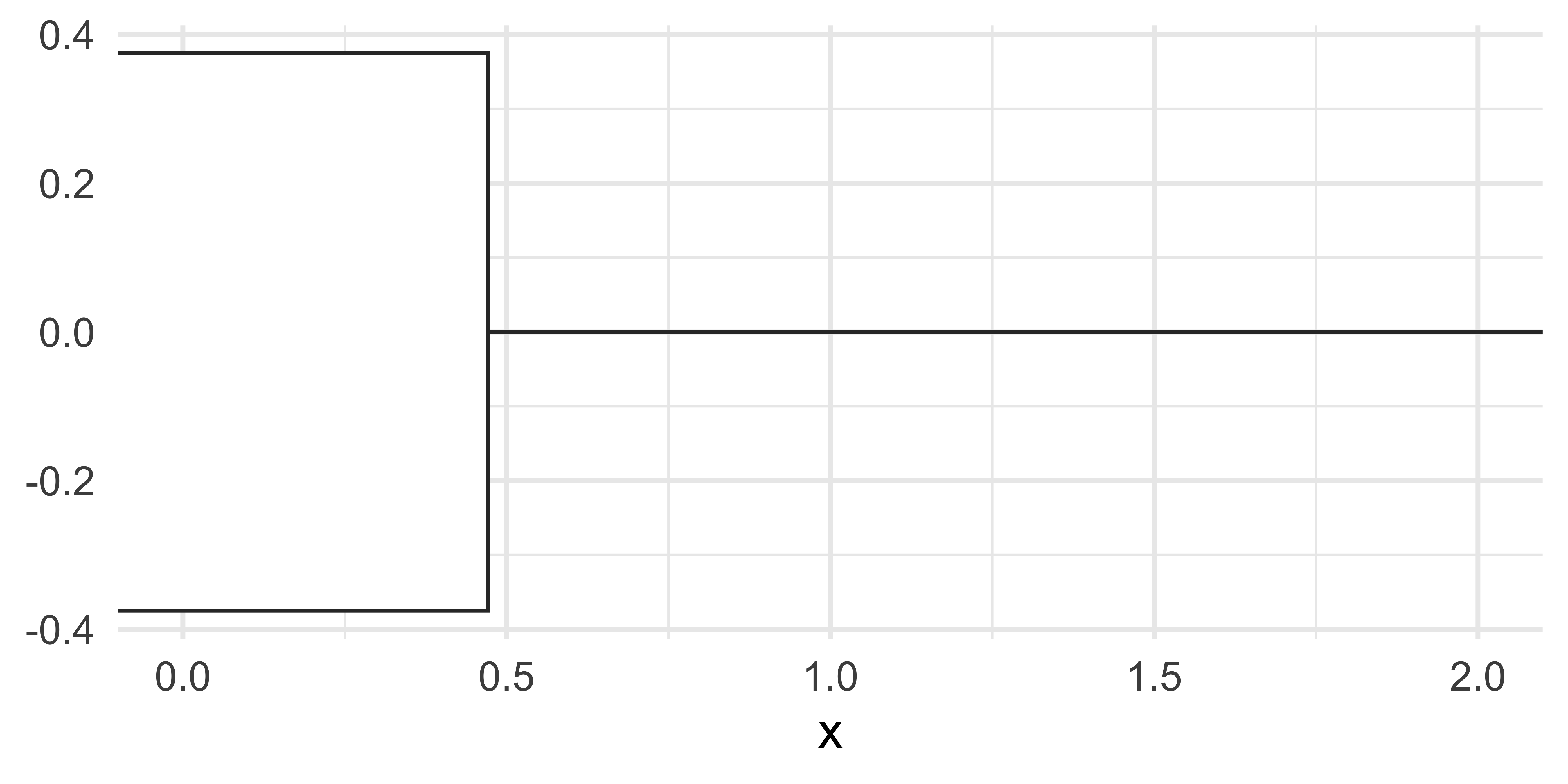
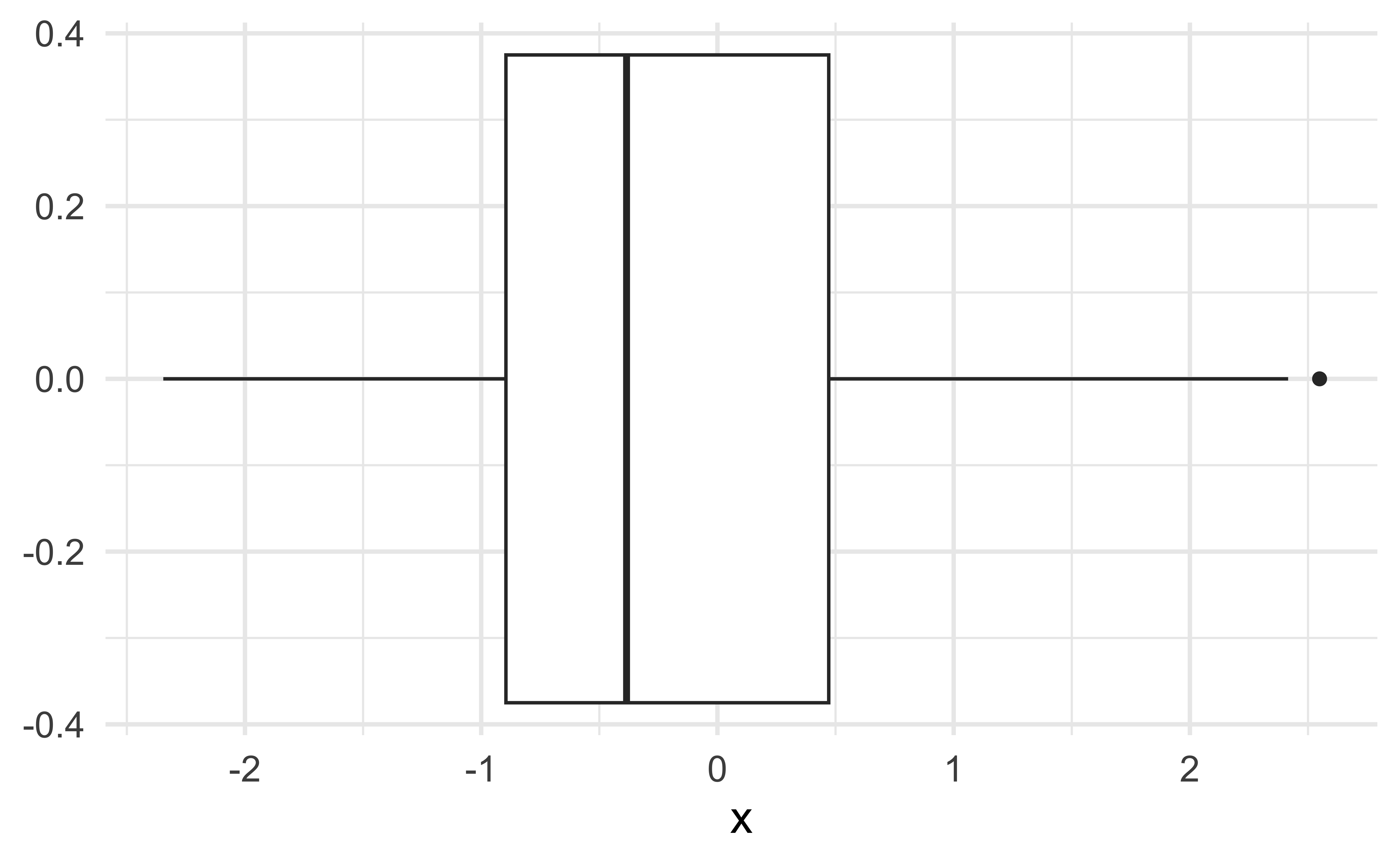
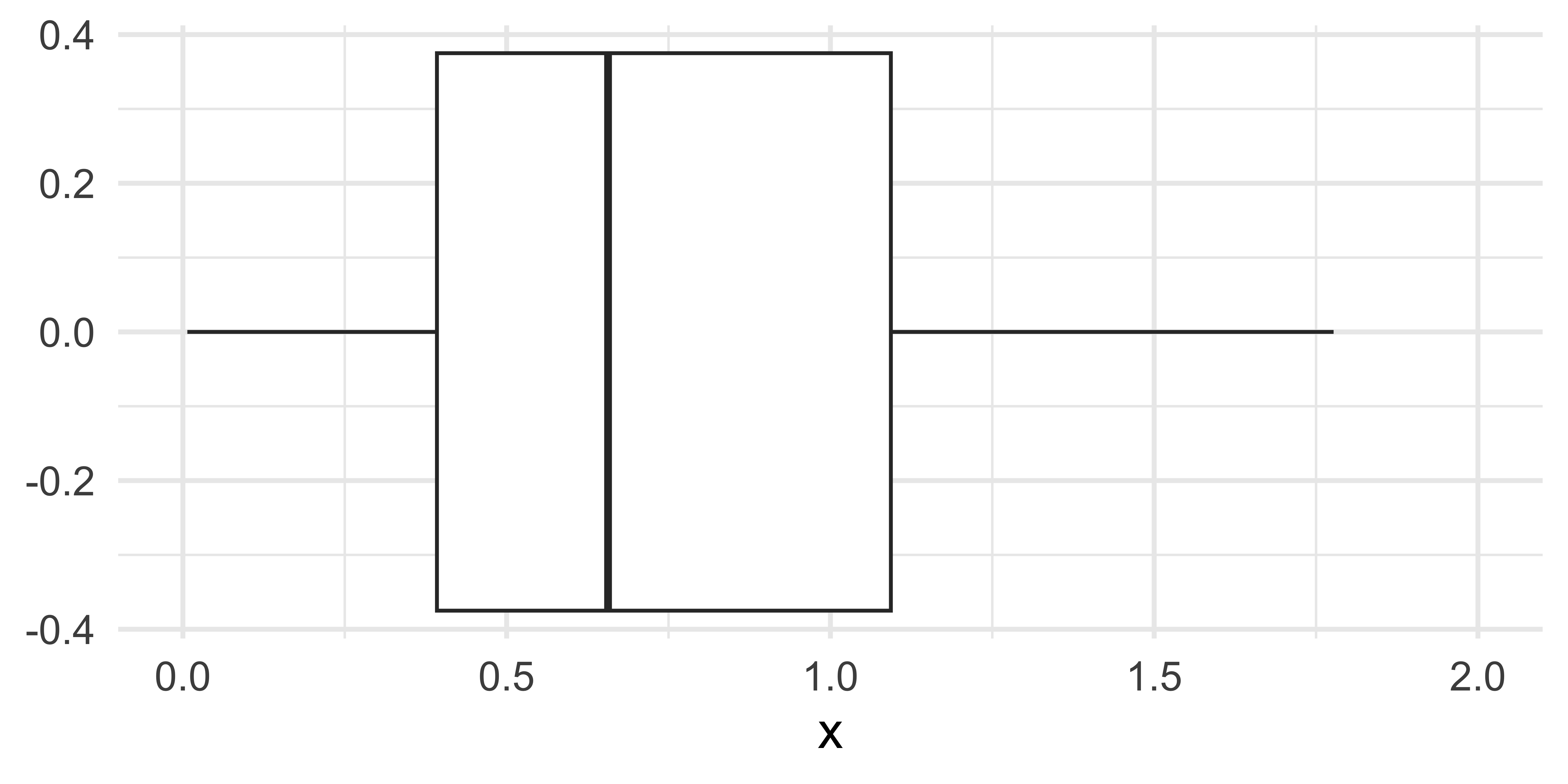
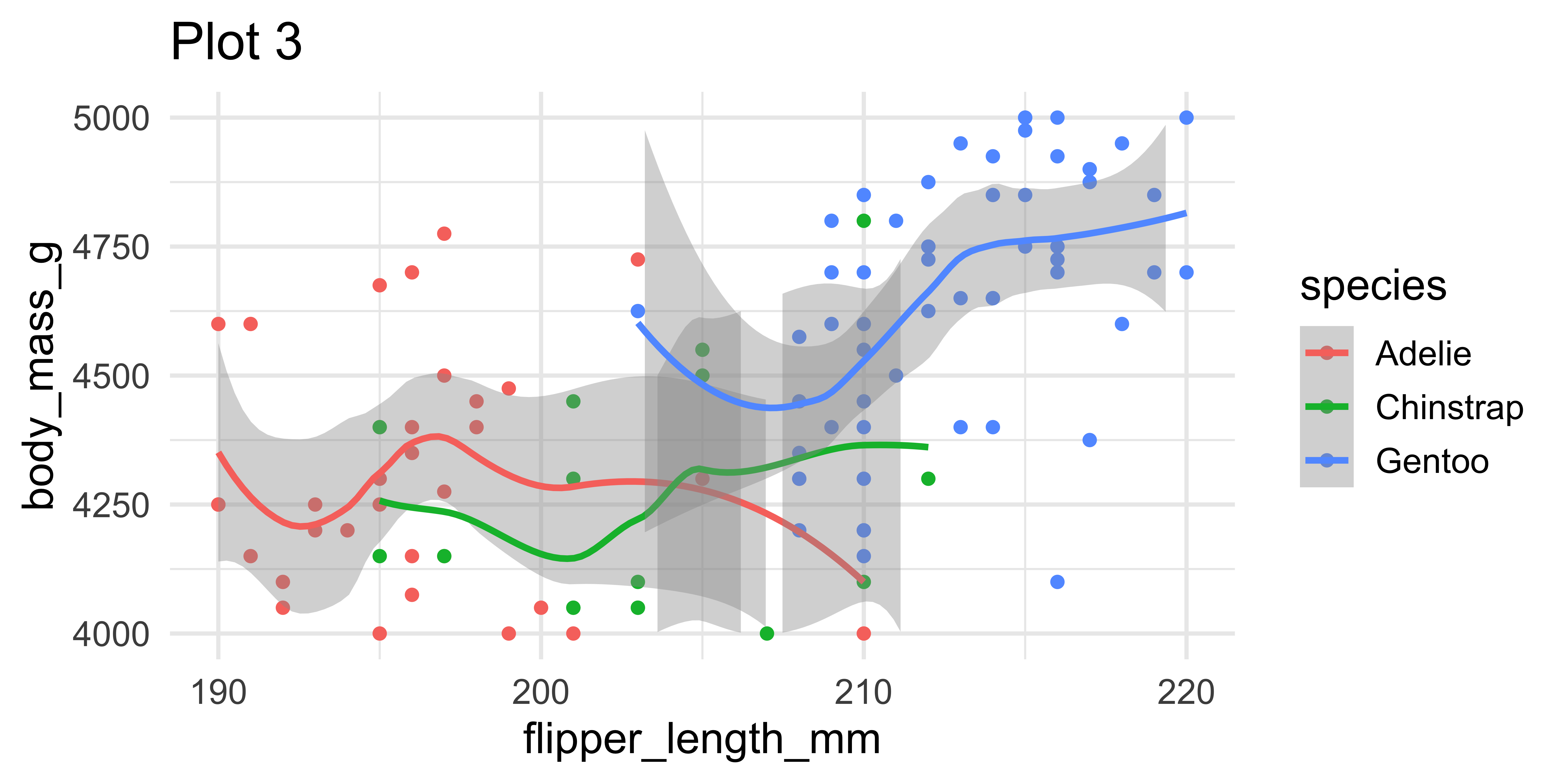
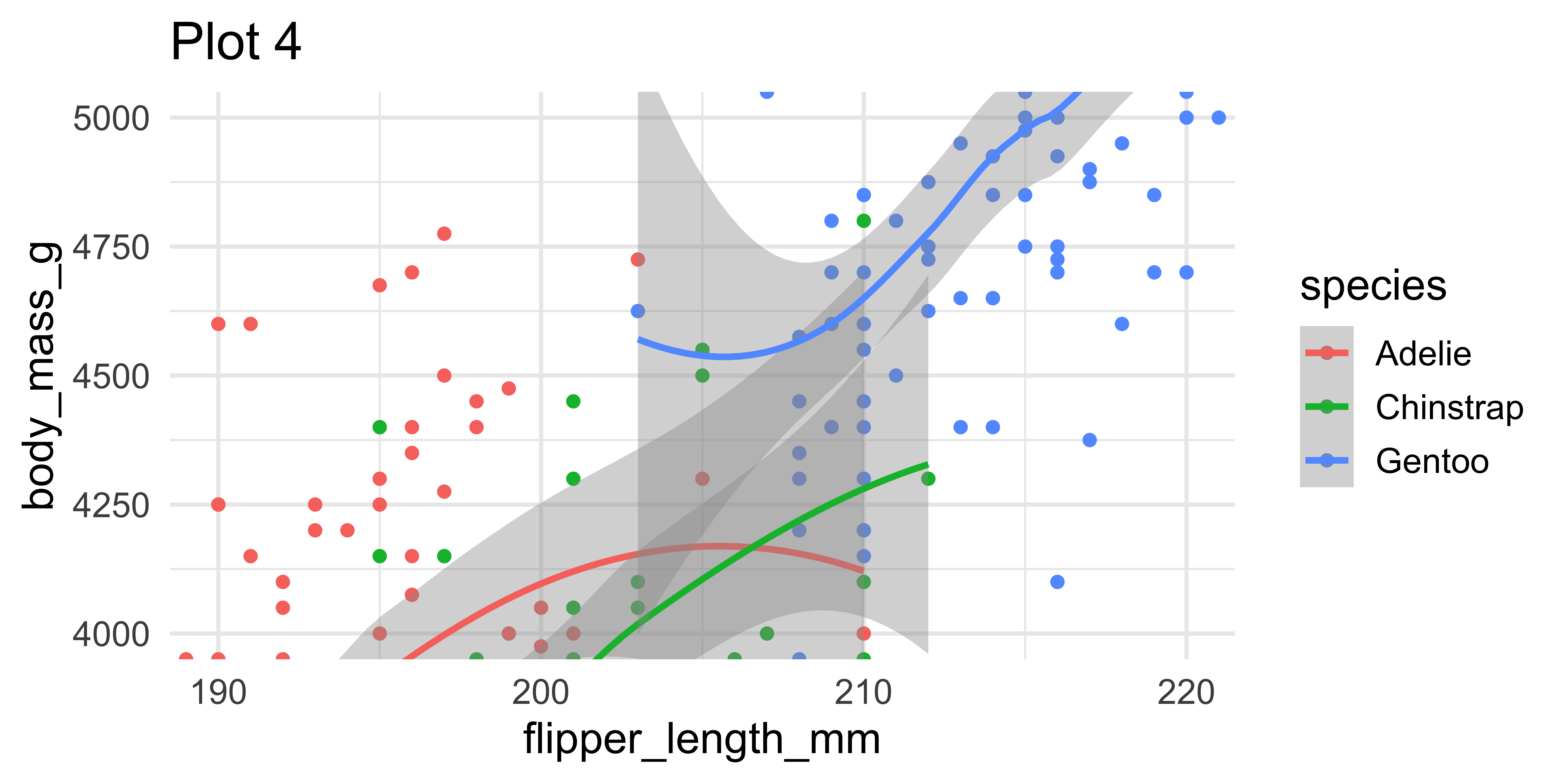
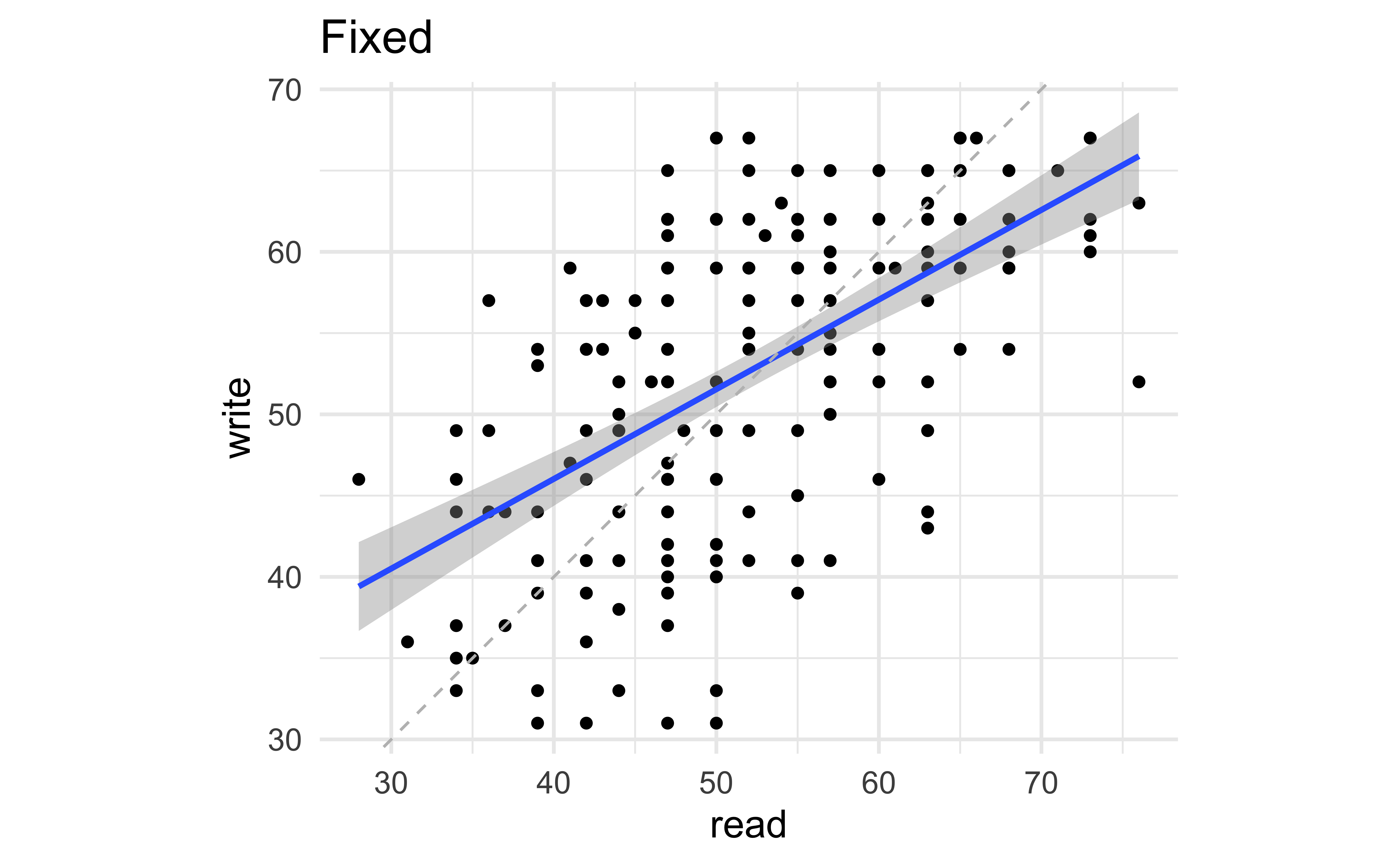
Setting limits: what the plots say

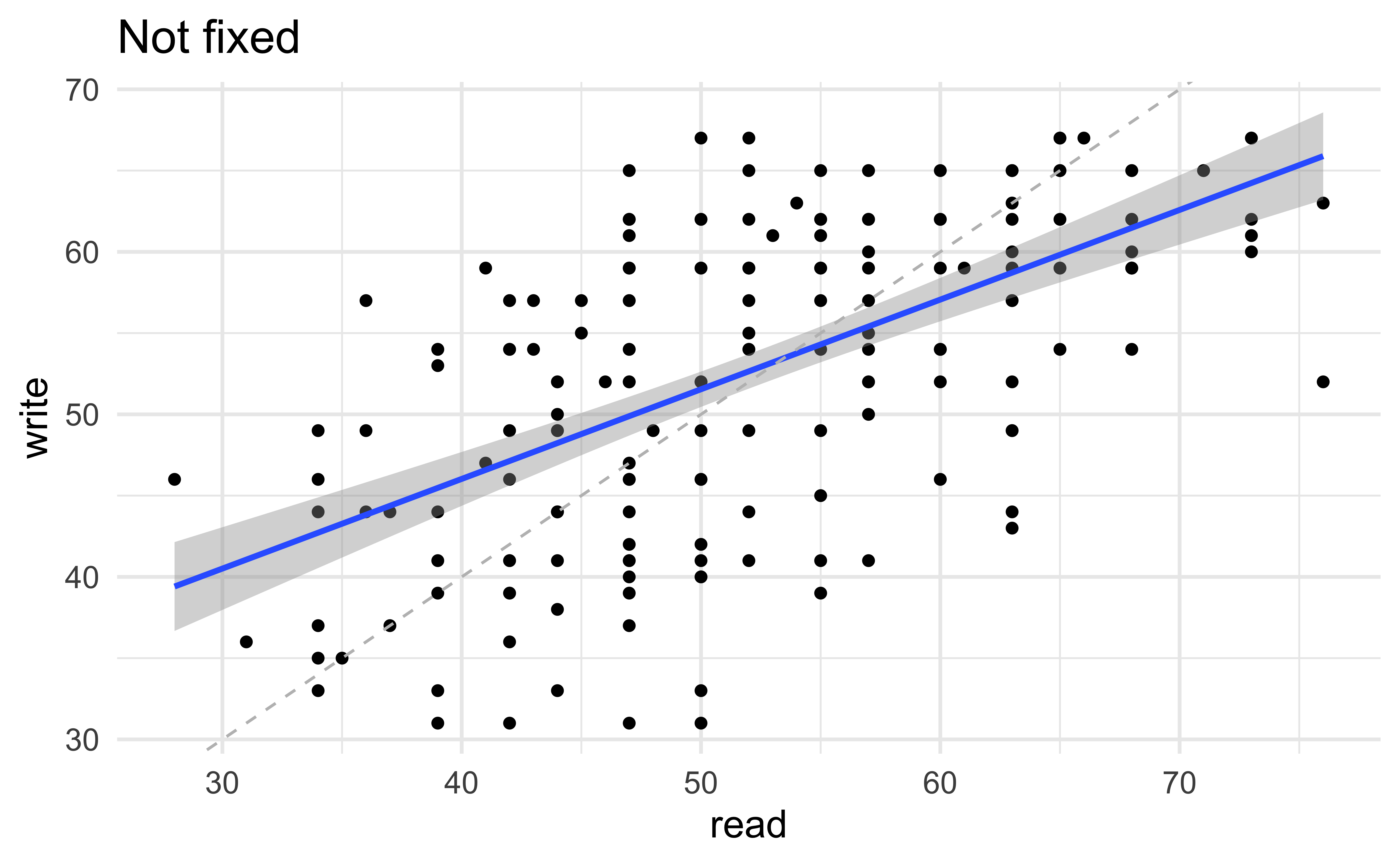
Fixing aspect ratio with coord_fixed()
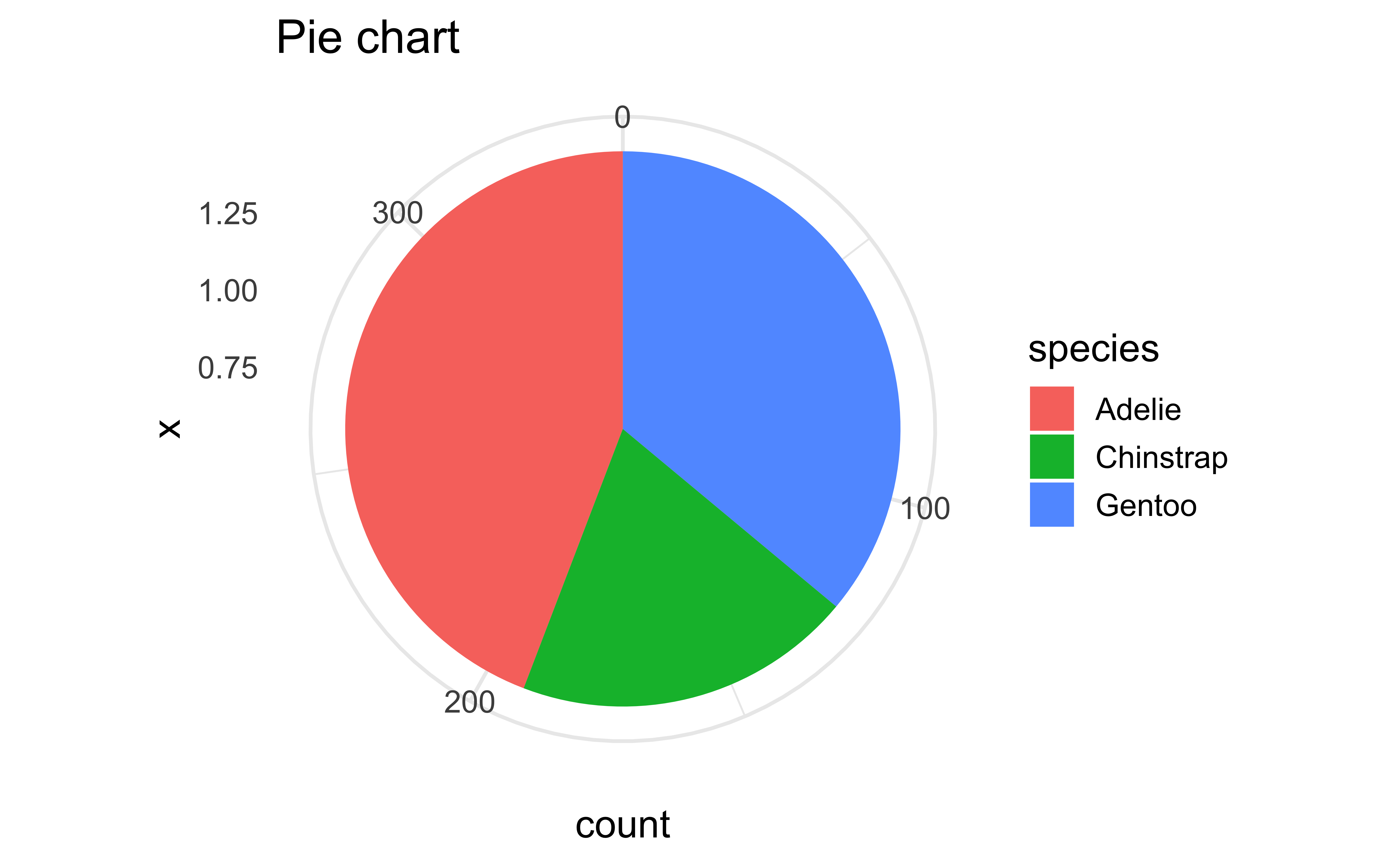
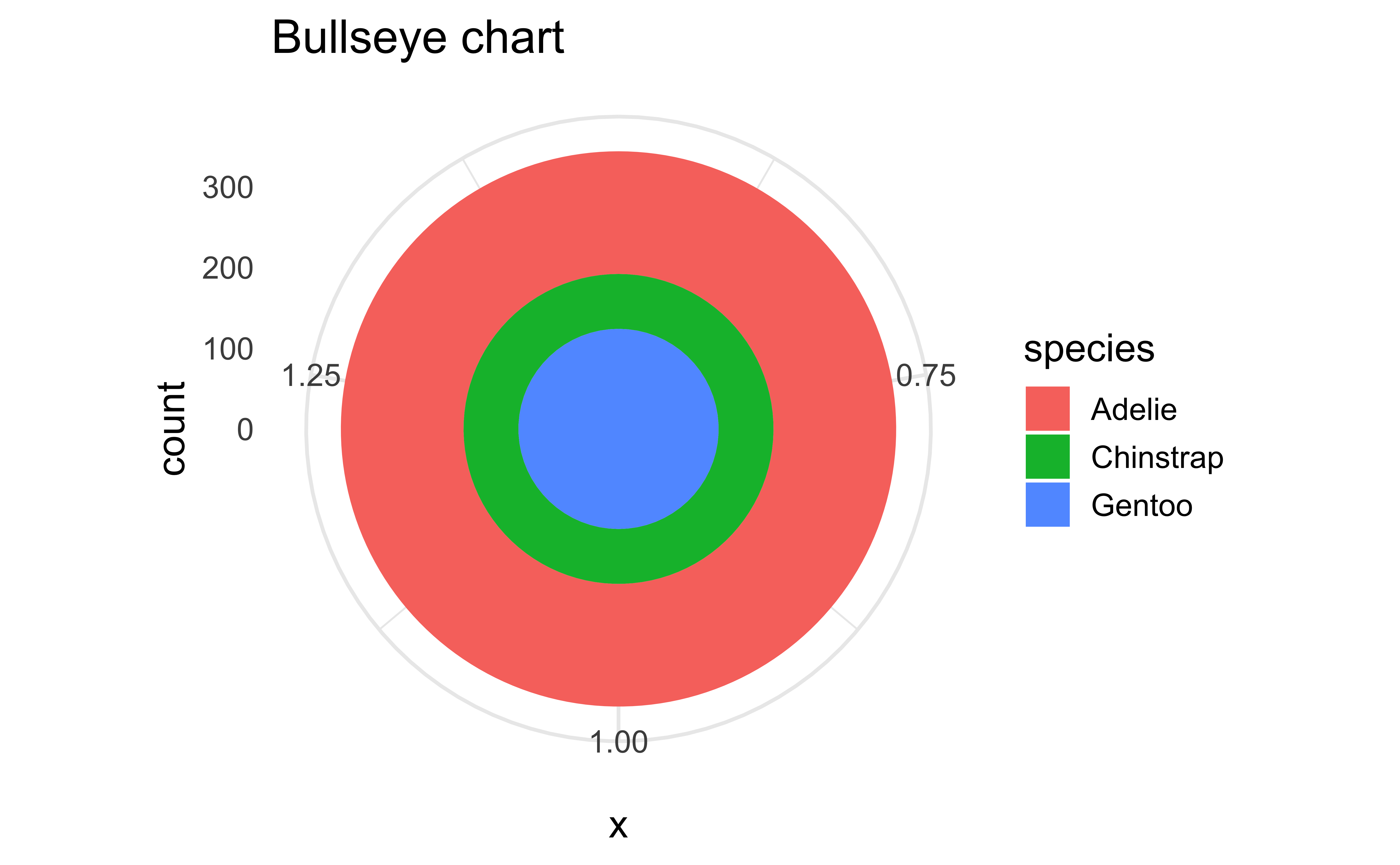
Pie charts and bullseye charts with coord_polar()
ggplot(penguins, aes(x = 1, fill = species)) +
  geom_bar() +
  labs(title = "Stacked bar chart")

ggplot(penguins, aes(x = 1, fill = species)) +
  geom_bar() +
  coord_polar(theta = "y") +
  labs(title = "Pie chart")

ggplot(penguins, aes(x = 1, fill = species)) +
  geom_bar() +
  coord_polar(theta = "x") +
  labs(title = "Bullseye chart")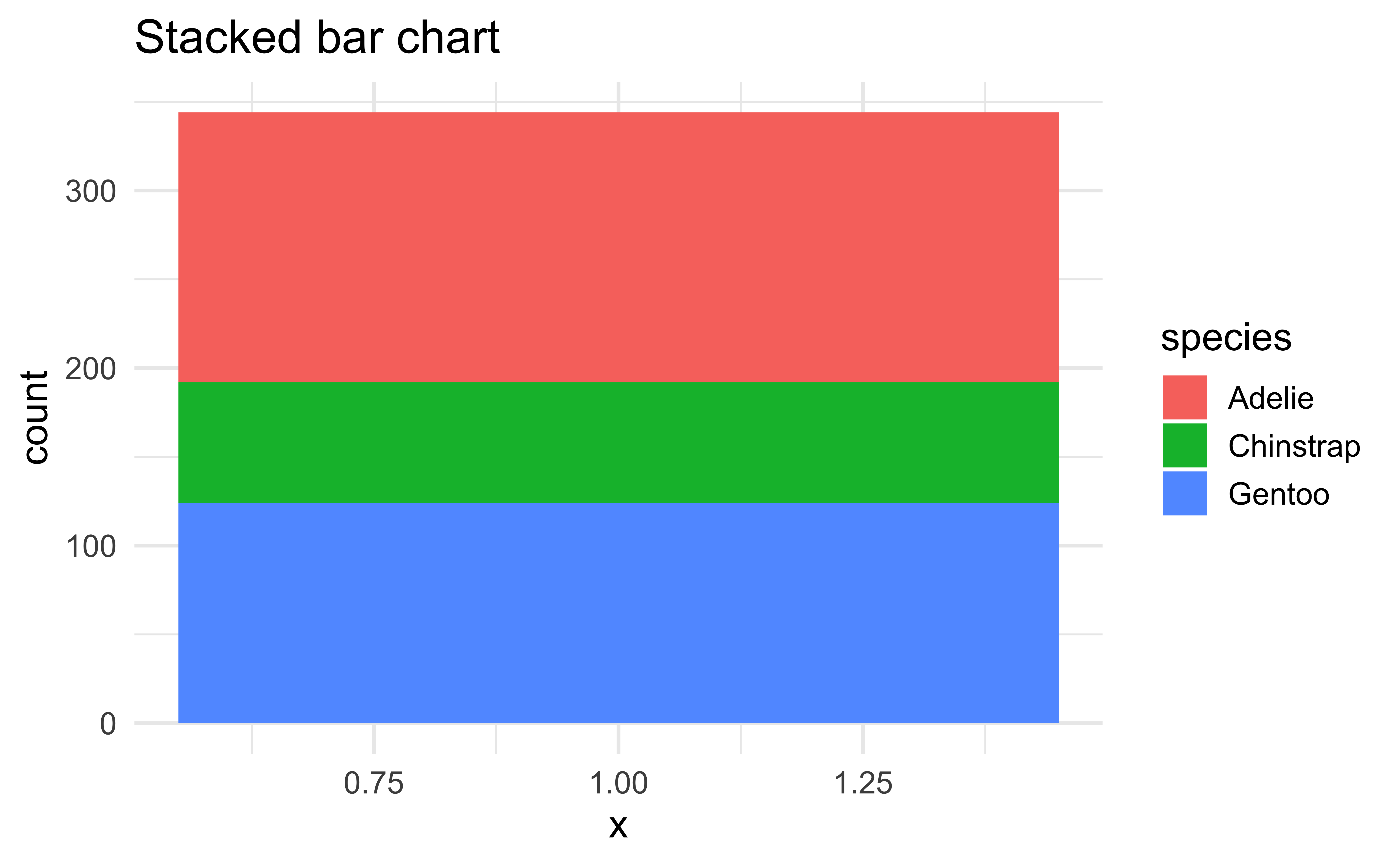
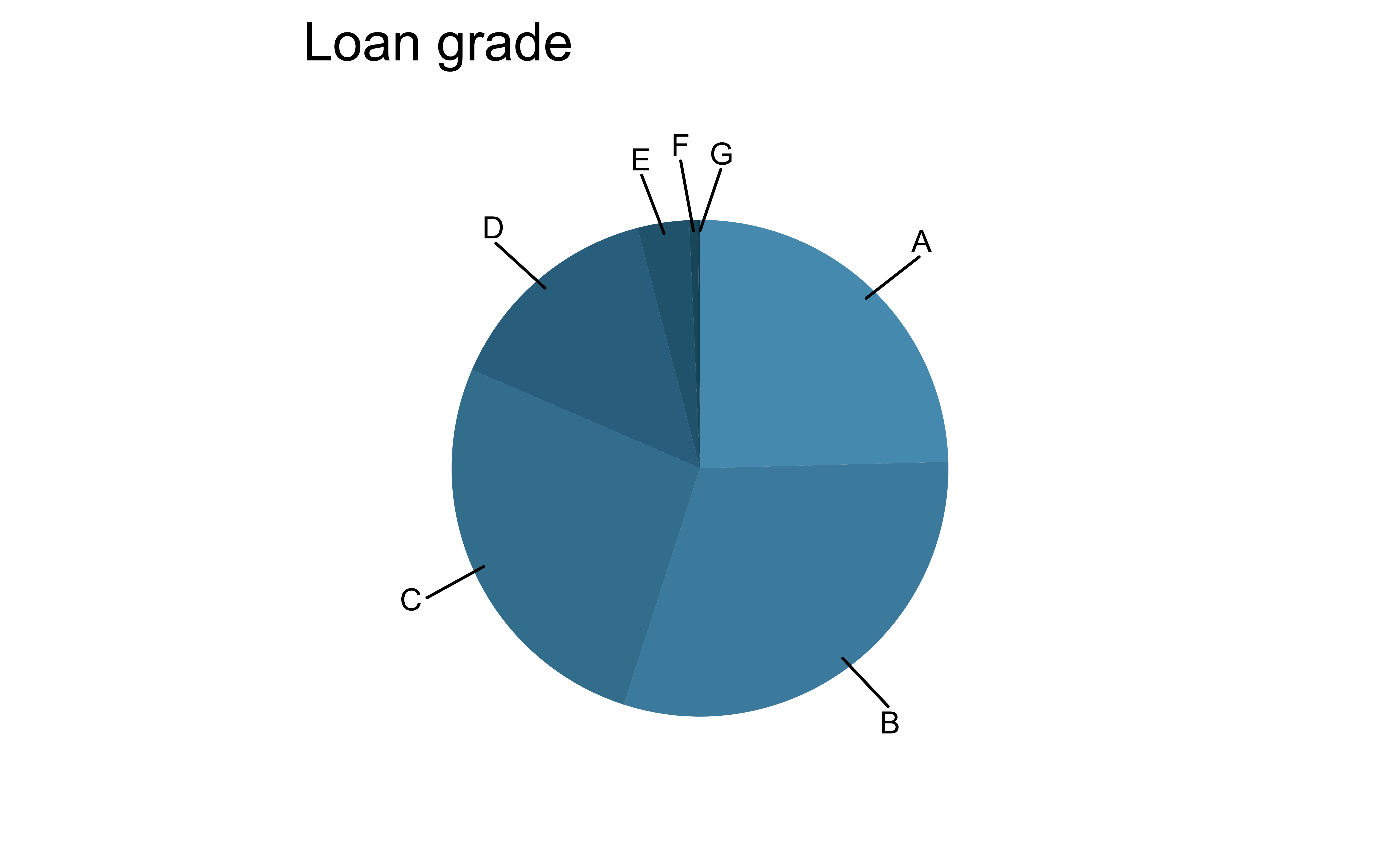
Pie charts
What do you know about pie charts and data visualization best practices? Love ’em or lose ’em?
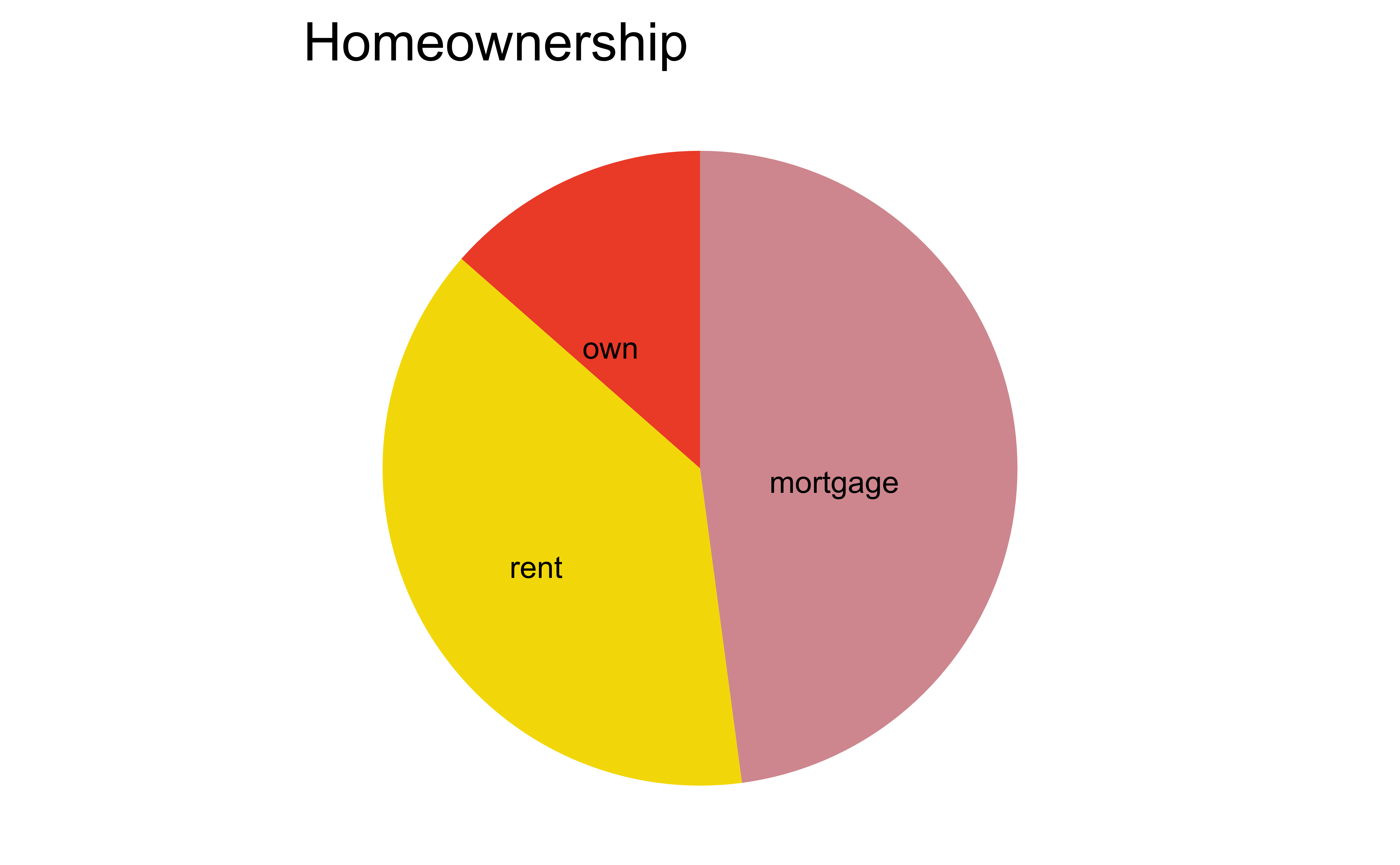
Pie charts: when to love ’em, when to lose ’em
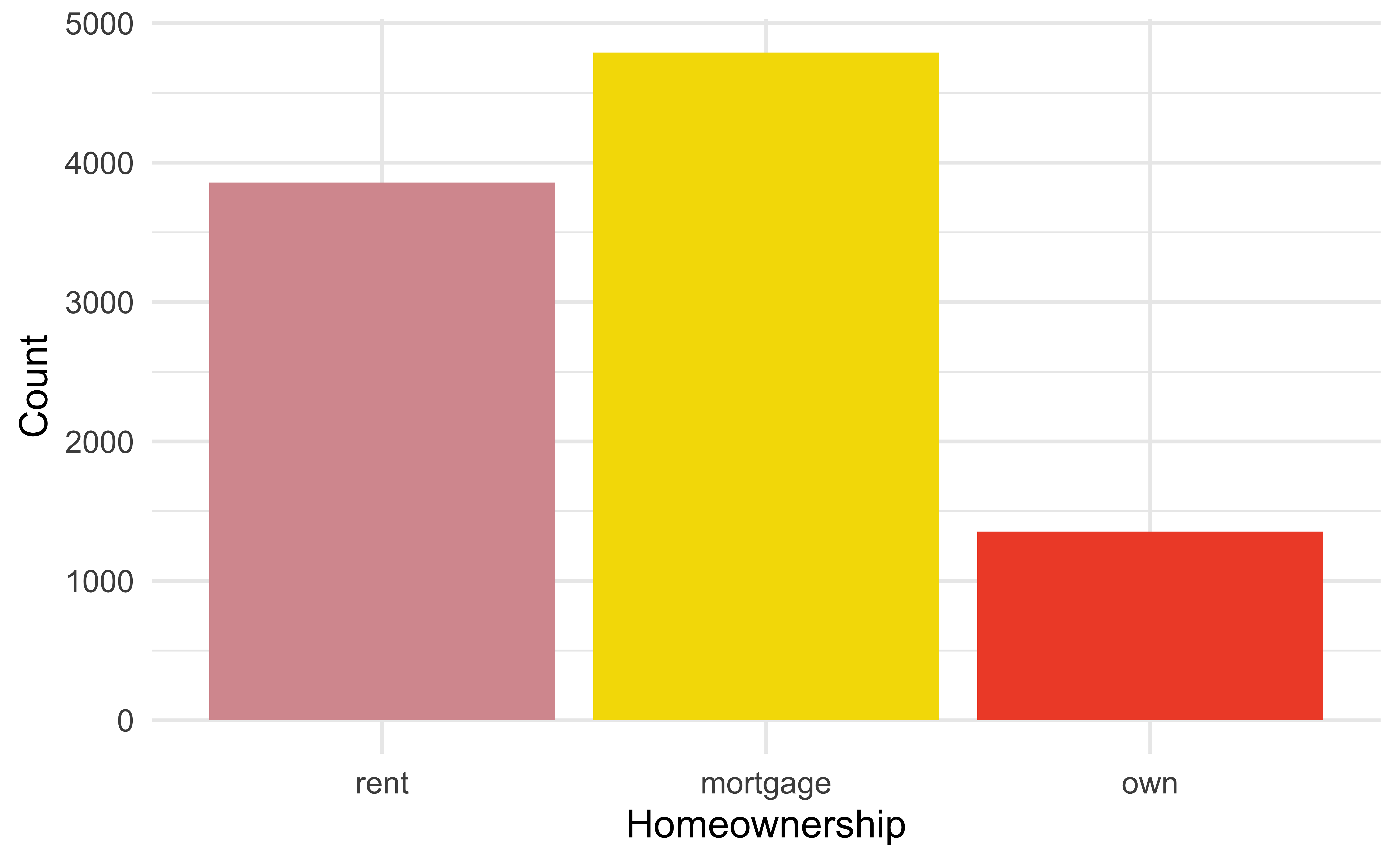
For categorical variables with few levels, bar charts can work well

Pie charts: when to love ’em, when to lose ’em
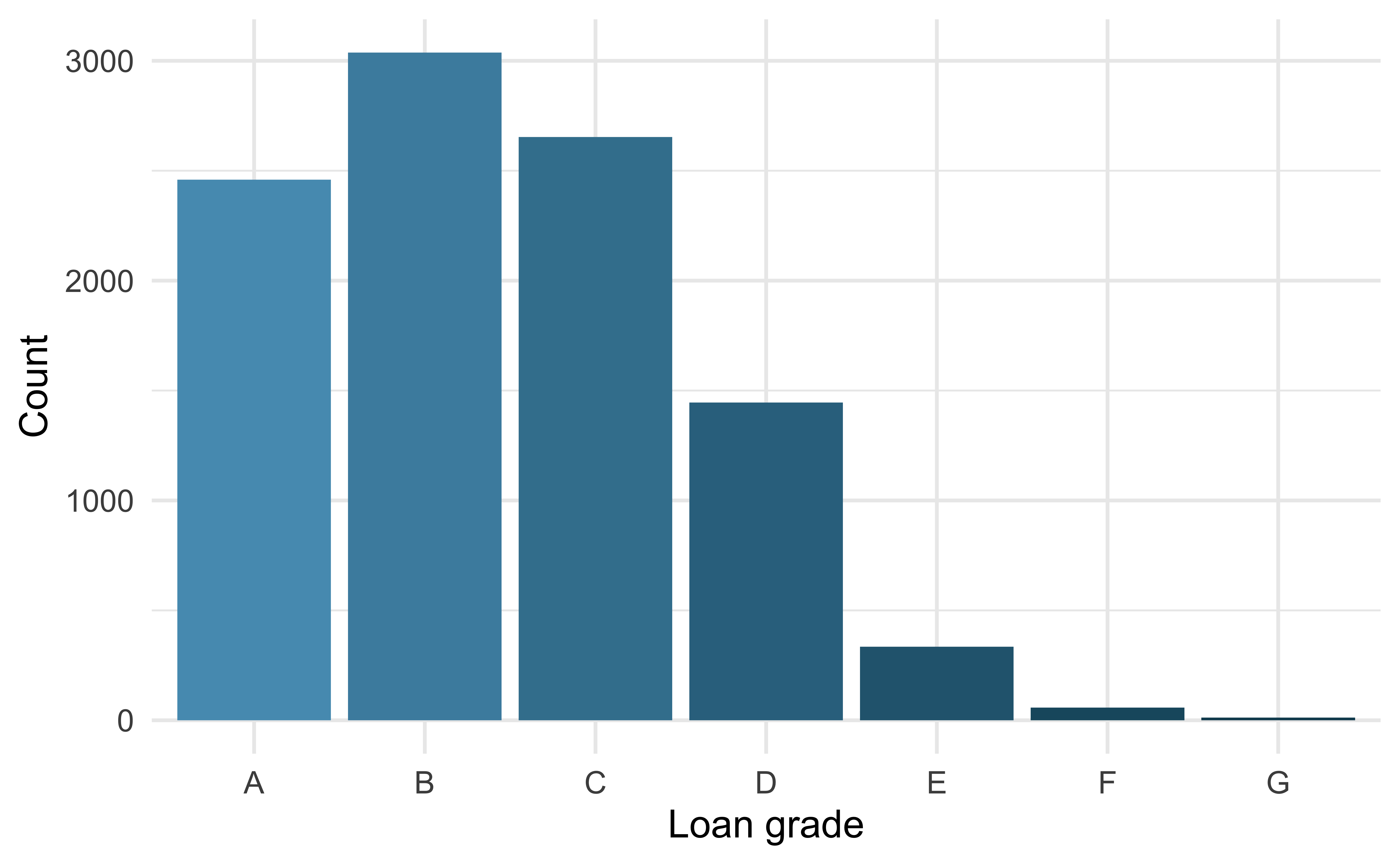
For categorical variables with many levels, bar charts are difficult to read

left_join()

right_join()

full_join()
inner_join()

semi_join()
anti_join()
Visualizing joined data
Livecoding
Reveal below for code developed during live coding session.
- Transform
Code
scientists_longer <- scientists |>
  mutate(
    birth_year = case_when(
      name == "Ada Lovelace" ~ 1815,
      name == "Marie Curie" ~ 1867,
      TRUE ~ birth_year
    ),
    death_year = case_when(
      name == "Ada Lovelace" ~ 1852,
      name == "Marie Curie" ~ 1934,
      name == "Flossie Wong-Staal" ~ 2020,
      TRUE ~ death_year
    ),
    status = if_else(is.na(death_year), "alive", "deceased"),
    death_year = if_else(is.na(death_year), 2021, death_year),
    known_for = if_else(name == "Rosalind Franklin", "understanding of the molecular structures of DNA ", known_for)
  ) |>
  pivot_longer(
    cols = contains("year"),
    names_to = "year_type",
    values_to = "year"
  ) |>
mutate(death_year_fake = if_else(year == 2021, TRUE, FALSE))- Plot
Code
ggplot(scientists_longer,
       aes(x = year, y = fct_reorder(name, as.numeric(factor(profession))), group = name, color = profession)) +
  geom_point(aes(shape = death_year_fake), show.legend = FALSE) +
  geom_line(aes(linetype = status), show.legend = FALSE) +
  scale_shape_manual(values = c("circle", NA)) +
  scale_linetype_manual(values = c("dashed", "solid")) +
  scale_color_colorblind() +
  scale_x_continuous(expand = c(0.01, 0), breaks = seq(1820, 2020, 50)) +
  geom_text(aes(y = name, label = known_for), x = 2030, show.legend = FALSE, hjust = 0) +
  geom_text(aes(label = profession), x = 1809, y = Inf, hjust = 1, vjust = 1, show.legend = FALSE) +
  coord_cartesian(clip = "off") +
  labs(
    x = "Year", y = NULL,
    title = "10 women in science who changed the world",
    caption = "Source: Discover magazine"
  ) +
  facet_grid(profession ~ ., scales = "free_y", space = "free_y", switch = "x") +
  theme(
    plot.margin = unit(c(1, 23, 1, 4), "lines"),
    plot.title.position = "plot",
    plot.caption.position = "plot",
    plot.caption = element_text(hjust = 2), # manual hack
    strip.background = element_blank(),
    strip.text = element_blank(),
    axis.title.x = element_text(hjust = 0),
    panel.background = element_rect(fill = "#f0f0f0", color = "white"),
    panel.grid.major = element_line(color = "white", size = 0.5)
  )